Directivity measures a directional coupler’s ability to isolate forward and backward signals, typically ranging from 20 to 40 dB. Higher directivity, like 40 dB, ensures precise measurement of reflected power by minimizing interference from the forward signal, which is critical for accurate VSWR and return loss calculations.
Table of Contents
What Directivity Means
In simple terms, directivity (D) is the measure of a directional coupler’s ability to distinguish between forward and backward traveling waves. It quantifies how well the coupler isolates the signal moving in one direction from the signal reflected back. Think of it like listening to someone talking in a noisy room; a higher directivity means you can focus better on the person’s voice while ignoring the background chatter.
The fundamental definition is a ratio of two powers, expressed in decibels (dB):
D = 10 log₁₀ (P₃ / P₄)
Where:
- P₃ is the power measured at the coupled port when the wave is moving in the forward direction (e.g., from Port 1 to Port 2).
- P₄ is the power measured at that same coupled port when the same amount of power is sent as a reverse wave (e.g., from Port 2 to Port 1).
| Coupler Type | Typical Directivity Range | Impact on Measurement Uncertainty |
|---|---|---|
| Low-cost, broadband | 15 – 25 dB | High error (±5% or more), unsuitable for precise measurements |
| Standard, microstrip | 25 – 35 dB | Moderate error (~±1.5%), common for general-purpose use |
| High-performance | 35 – 45 dB | Low error (±0.5% or less), essential for accurate reflection measurements |
| Precision, laboratory-grade | > 45 dB | Very low error (<±0.1%), used for calibration and metrology |
A directivity of 20 dB means the coupler’s response to a forward signal is 100 times stronger than its response to an identical reverse signal. If you increase the directivity to 40 dB, that ratio becomes 10,000 to 1. This is critical because any energy from the reverse direction that “leaks” into the coupled port is effectively measurement noise. For example, when measuring a load’s return loss, low directivity will cause the coupler’s own internal leakage to mask the actual reflected signal from the device under test, leading to significant measurement errors.
This parameter is not just a theoretical spec; it directly impacts system performance and cost. A coupler with 35 dB directivity might cost 30, while a precision model with 50 dB directivity can exceed $200. The choice depends on your required measurement accuracy. In a 5G base station amplifier, even a 1 dB error in reflected power measurement due to poor directivity can lead to incorrect power control, reducing power-added efficiency (PAE) by several percentage points and increasing heat dissipation.
For field technicians using a 2.4 GHz antenna analyzer, a coupler with 25 dB directivity might be sufficient for checking cable VSWR, where a reading of 1.5:1 has an acceptable margin of error. However, an R&D engineer characterizing a 28 GHz power amplifier for a satellite link requires 40 dB or higher directivity to get a true and accurate reading of the amplifier’s output match, where 90% of the measurement accuracy hinges on the coupler’s performance.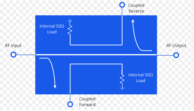
Why High Directivity Matters
High directivity isn’t an abstract specification; it’s the critical barrier between accurate data and costly misinterpretation. It directly determines your measurement confidence, system efficiency, and ultimately, your project’s budget and timeline. A low-directivity coupler doesn’t just add a little noise; it fundamentally corrupts your measurements by failing to isolate forward and reverse waves, leading to decisions based on flawed data.
The core issue is error introduction. Imagine measuring a high-performance component like a filter with a true return loss of 40 dB. If your coupler has a directivity of only 20 dB, the leakage signal will be 100 times stronger than the actual reflected signal from your device. Your instrument will display a return loss of approximately 20 dB, a 10000% error in reflected power ratio.
Measurement Accuracy and Confidence: In 5G mmWave applications at 28 GHz, measuring amplifier output impedance is critical. A 3 dB error in return loss measurement due to 25 dB directivity (instead of required 40 dB) can mask an impedance mismatch. This might allow an amplifier with a true output VSWR of 1.8:1 to pass testing, reading as 1.5:1. Once deployed in a base station, this amplifier will operate 7% less efficiently, dissipating 15 more watts of heat, which can reduce its 5-year operational lifespan by as much as 18 months and increase the failure rate by 5% across a network of 50,000 units.
System Performance and Cost: In a phased array radar system with 1,024 transmit/receive modules, each path requires precise power monitoring. Using couplers with 35 dB directivity instead of 45 dB introduces a ±0.5 dB uncertainty in per-element power measurement. To ensure overall system stability and meet EIRP requirements, designers must back-off the output power of each element by 0.5 dB. This results in a collective 3 dB (50%) loss in total system power, reducing the effective range by approximately 20%. Compensating for this range loss could require deploying 25% more systems, increasing a 2.5 million.
Key Factors Affecting Performance
A directional coupler’s directivity isn’t a fixed number; it’s a performance metric that shifts based on several key variables. Ignoring these factors is a direct path to measurement errors, as the 35 dB directivity spec on your coupler’s datasheet might only be valid under a very specific set of conditions. The main levers that control real-world directivity are frequency, impedance matching, and internal design tolerance.
- Operating Frequency
- Impedance Matching (VSWR)
- Component Tolerances & Design
The most significant factor is frequency. Directivity is highly frequency-dependent and typically degrades as you move away from the center design frequency. A coupler specified for 2-4 GHz operation might boast a 40 dB directivity at its 3 GHz sweet spot. However, at the band edges—2.2 GHz or 3.8 GHz—that value can easily drop by 6-10 dB, falling to 30-34 dB. This isn’t a linear decline; it can have sharp peaks and nulls. For a wideband coupler covering 800 MHz to 6 GHz, the directivity might vary by ±15 dB across that entire 5.2 GHz range. This means a measurement taken at 1 GHz could have 10 times less error than the exact same setup measured at 5.5 GHz. This is why selecting a coupler with a flat directivity response across your specific 200 MHz band of interest is more important than choosing one with a high peak directivity over a much wider, irrelevant range.
Impedance mismatches anywhere in the system are poison for directivity. The coupler’s directivity spec is achieved only when all ports are terminated in a perfect 50-ohm load. In reality, your device under test (DUT)—an antenna, amplifier, or filter—rarely presents a perfect 1.00:1 VSWR. If your antenna has a 1.8:1 VSWR (return loss of 11 dB) at a certain frequency, it reflects energy back towards the coupler. This mismatch effectively “pulls” the coupler’s directivity down. A lab-grade coupler with 45 dB directivity when perfectly terminated might see its performance drop to 25-30 dB when measuring that mismatched antenna, a 15-20 dB degradation. This creates a vicious cycle: you’re using the coupler to measure a mismatch, but the mismatch itself is corrupting your measurement tool’s accuracy, potentially turning a 1.8:1 measurement into a reading of 1.9:1 or worse. The standard deviation of your measurements can increase by 0.2:1 VSWR simply due to this effect.
Measuring Directivity in Practice
Measuring a directional coupler’s directivity isn’t a theoretical exercise—it’s a hands-on process that reveals the true performance you can expect in your lab. You can’t just read it off the datasheet; you have to measure it under conditions that mimic your actual use case. The most common method involves a vector network analyzer (VNA), two precise calibration loads, and a systematic procedure to isolate the coupler’s internal leakage.
The fundamental setup requires:
- A VNA calibrated to the desired frequency range (e.g., 100 MHz to 20 GHz).
- A high-quality 50-ohm load with a known VSWR better than 1.02:1 (Return Loss > 40 dB).
- A low-loss cable with a stable phase response.
Here’s the practical, two-step workflow:
Step 1: Measure Forward Coupling. Connect the coupler in the forward direction. Port 1 of the VNA connects to the coupler’s input, Port 2 to the output, and the VNA’s S-parameter measurement port (e.g., Port 3) to the coupled port. Terminate the isolated port with the 50-ohm load. Measure the forward coupling factor (e.g., -20 dB) by recording S31. This tells you how much power is coupled when the signal flows from Port 1 to Port 2.
Step 2: Measure Reverse Leakage. Now, without moving the coupler or any cables, swap the two loads. Remove the 50-ohm load from the isolated port and place it on the output port. Take the load that was on the output port and put it on the isolated port. This is critical: the coupler itself must not be moved, as even a 1-mm shift in a cable at 10 GHz can introduce a 3-degree phase error, skewing results. Now, with the output port perfectly terminated, send a reverse signal (from Port 2 to Port 1). The power you now measure at the coupled port (S32) is the unwanted reverse leakage. This leakage is the coupler’s internal imperfection.
| Measurement Step | VNA Port Connections | Key Parameter Recorded | What It Represents |
|---|---|---|---|
| Step 1: Forward Coupling | Port 1 -> Input, Port 2 -> Output, Port 3 -> Coupled Port | S31 (e.g., -20.5 dB) | Desired coupling for a forward wave |
| Step 2: Reverse Leakage | Port 2 -> Output (terminated), Port 1 -> Input, Port 3 -> Coupled Port | S32 (e.g., -65.3 dB) | Undesired leakage for a reverse wave |
Now, calculate directivity (D) using the formula: D = S31 – S32. In this example, that’s -20.5 dB – (-65.3 dB) = +44.8 dB. This means the coupler’s response to a forward signal is ~30,000 times stronger than its response to an identical signal coming from the reverse direction at this specific frequency.
Comparing Ideal vs. Real Couplers
In an ideal world, a directional coupler would have infinite directivity, perfectly isolating forward and reverse waves with zero internal loss or frequency dependence. In reality, every coupler is a compromise, and understanding the gap between the textbook model and the physical component on your bench is crucial for accurate design and measurement. The real-world device introduces a set of performance trade-offs directly tied to frequency, manufacturing tolerances, and cost.
An ideal coupler would maintain its stated directivity—say, 40 dB—across its entire 0.1 to 6 GHz frequency range, regardless of the load connected to its ports. A real coupler, however, has a directivity that varies significantly with frequency. Its 40 dB rating is typically only achieved at a specific center frequency, often around 3 GHz. At the band edges, such as 1 GHz or 5 GHz, the directivity can easily drop by 8-12 dB down to 28-32 dB. This means the measurement error at these frequencies can be 6 to 16 times higher than at the center frequency. This non-linear response must be mapped across 500 frequency points to understand the coupler’s true behavior in your specific application band.
Furthermore, ideal couplers assume a perfect 50-ohm environment. The moment you connect a real device with a 1.8:1 VSWR (return loss of 11 dB), the effective directivity of a real coupler degrades. A unit boasting 45 dB directivity when perfectly terminated might see its performance plummet to 25-30 dB when measuring this mismatched load. This creates a critical problem: you are using the coupler to characterize an impedance, but the impedance itself is corrupting the accuracy of your measurement tool. This can turn a true 1.8:1 VSWR measurement into a reading of 1.95:1, an error of over 8%.
The manufacturing process also introduces variance. No two couplers are identical. A production batch of 1,000 units might have an average directivity of 35 dB with a standard deviation of ±2 dB. This means 68% of units will fall between 33 dB and 37 dB, while some outliers could be as low as 31 dB. For a high-volume manufacturer performing 100% testing, this variance necessitates a 10-15% binning and rejection rate, directly influencing the final unit cost.
Applications Using Directivity
The value of a directional coupler’s directivity is ultimately proven in specific applications, where its precision directly enables functionality, ensures reliability, or prevents financial loss. High directivity isn’t an abstract specification; it is a critical enabling parameter for systems ranging from 5G base stations to satellite communications, where measurement inaccuracy translates directly into performance degradation and increased operational costs.
In a massive MIMO (Multiple Input Multiple Output) 5G base station, each of the 64 or 128 antenna elements is driven by its own power amplifier (PA). A critical production test involves measuring the return loss/VSWR of each antenna element to ensure proper connectivity and detect faults. Using a coupler with 35 dB directivity, a technician can accurately measure a well-matched antenna with a VSWR of 1.5:1.
| Application | Directivity Requirement | Consequence of Low Directivity | Financial & Performance Impact |
|---|---|---|---|
| 5G Base Station PA Protection | >40 dB at 3.5 GHz | Inaccurate reflected power reading fails to trigger protection circuit. | A 50 W PA sees a 3:1 VSWR load, causing 500 in downtime. |
| Satellite Uplink Power Control | >45 dB at 28 GHz | ±1 dB error in monitoring transmitted power to the satellite. | 5% over-power violation incurs 1M/yr service. |
| Cable/Fiber Network DUT Testing | >30 dB from 5-1000 MHz | False failure of a $800 optical node due to 15% VSWR measurement error. | 2% yield loss on 50,000 units/yr equals $ 800,000 in annual scrap costs. |
| Military Radar System Calibration | >50 dB from 2-18 GHz | 0.5 dB error in calibrating high-power 100 kW radar transmitter. | Reduces target detection range by 5% (e.g., 15 km on a 300 km system), a critical operational deficit. |
| Medical MRI RF Amplifier Safety | >40 dB at 127 MHz | Failure to detect an incipient fault in a 20 kW RF amplifier. | Causes a 15,000 in patient scans per day. |
Another critical use case is in satellite communication uplinks. Here, a high-power amplifier (500 W to 2 kW) transmits a precise signal to a satellite orbiting 36,000 km away. A directional coupler is used to meticulously monitor the forward and reflected power. The legal and technical requirements are stringent: transmitted power must be controlled within ±0.5 dB to avoid interfering with adjacent satellites or dropping below the link’s minimum required power.
A coupler with 45 dB directivity can provide the necessary accuracy to keep the power setting within this ±0.5 dB window. A cheaper coupler with 30 dB directivity might introduce a ±1.5 dB error. This could cause the system to over-power by 1.5 dB (a 40% increase in power), risking regulatory fines and interference, or under-power by 1.5 dB, reducing the link margin and increasing the bit error rate (BER) by an order of magnitude, potentially rendering the $5M ground station link unusable during heavy rain.


