What Are Broadband Omni Waveguide Antennas For

Broadband omni waveguide antennas serve multi-directional, wide-frequency comms—e.g., covering 2-18GHz, they enable base stations/ radar to radiate uniformly, handling signals from Wi-Fi to satellite links without directional adjustment for flexible connectivity.

Wireless Communication Systems

In 2023, the total number of 5G base stations in China exceeded 3.37 million (data from the Ministry of Industry and Information Technology), and IoT connections surpassed 2 billion (GSMA report). Wireless communication systems are facing the dual challenge of “wide coverage + multi-band”.

Traditional omnidirectional antennas commonly suffer from three major pain points: narrowband limitations (e.g., only supporting n41/n78 dual bands, covering 1710-2690MHz), mechanical rotation delay (0.5-2 seconds to align with signal source), and high multi-band deployment cost (requiring 3-4 antennas per site, increasing total cost by 30%).

Broadband omnidirectional waveguide antennas, with their 698-6000MHz ultra-wideband coverage (10:1 bandwidth ratio), non-mechanical omnidirectional radiation (3dB beamwidth >320°), and 25% lower per-site cost (compared to traditional combinations), have become key equipment for solving the challenges of “dead-zone-free connectivity + multi-generation communication compatibility”.

Technical Principle

Ordinary dipole antennas have a bandwidth of at most 20% (e.g., a 4G antenna covering 700-960MHz), with a gain of less than 2 dBi during omnidirectional radiation. Parabolic antennas have slightly better bandwidth (30%), but their beam is as narrow as a flashlight, losing signal when direction changes.

Broadband omnidirectional waveguide antennas aim to break this contradiction:can cover 698-6000MHz (10:1 bandwidth ratio, equivalent to the span from FM radio to satellite communication), with a horizontal plane 3dB beamwidth compressed to over 320°, achieving almost “dead-zone-free” coverage.

The “Basic Model” of Waveguide: First Understand This Metal Tube

A waveguide is essentially a hollow metal tube (commonly aluminum alloy, wall thickness 1mm, lightweight and corrosion-resistant), often with a rectangular cross-section. Its core function is “wave guidance” – it only allows electromagnetic waves of specific frequencies to propagate inside; waves outside the range are reflected back.

For example, the antenna we use has a waveguide wide side a=10mm, height b=3mm. Using the formula f_c = c/(2a√ε_r) (where c is the speed of light, 3e8 m/s, ε_r is the dielectric constant, approximately 1 for air), the cutoff frequency is calculated to be about 15 GHz.

How is Broadband “Spread Out”? Relies on “Speed Bumps” and a “Mixing Console” on the Inner Wall

Relying solely on the waveguide itself, bandwidth might only reach around 10 GHz. To cover up to 6 GHz or higher, the inner wall must be modified. We etched gradual impedance helical grooves on the inner wall of the waveguide: groove depth gradually changes from 0.2mm to 0.7mm, pitch is 1.2mm, total length occupying one-third of the waveguide. This design is like installing “speed bumps” for electromagnetic waves – high-frequency signals (e.g., 6 GHz) attenuate slowly in deep grooves, low-frequency signals (e.g., 700 MHz) reflect less in shallow grooves, allowing both to pass through smoothly.

Another key design is ridge loading: a metal ridge 0.5mm high is added to the center of the waveguide’s wide side. the effective width of the TE10 mode increases, its cutoff frequency drops to 5 GHz, while simultaneously suppressing the premature appearance of the TE20 mode. Tests show that after adding the ridge, the gain fluctuation in the frequency band below 5 GHz shrinks from ±1.5 dBi to ±0.8 dBi (smaller fluctuation means more uniform omnidirectional coverage).

How is Omnidirectional “Evened Out”? Making Directional Waves “Hit the Wall” and Become Circular

Waveguides naturally tend to propagate in straight lines; the output port has a narrow beam (e.g., traditional waveguide antenna 3dB beamwidth is only 60°). To achieve omnidirectional radiation, the energy in the waveguide must be redistributed after “hitting a wall.” We connected a gradual flared horn to the waveguide outlet: the aperture gradually changes from 20mm×6mm to 100mm×30mm, with a length of 150mm.

Even more ingenious is mode superposition: allowing the TE10 mode and TM01 mode to interfere at the horn aperture. The TE10 mode is primarily horizontally polarized, the TM01 mode is primarily vertically polarized; their superposition forms circular polarization (axial ratio <3dB). This polarization method has strong resistance to multipath fading – between urban high-rises, signal reflections generate positive and negative polarized waves; circular polarization can cancel them out.

Hard Data Speaks: How Capable is This Structure?

• Power Capacity: Aluminum alloy waveguide wall thickness 1mm, calculated power capacity is 500W (continuous wave), 2.5 times that of traditional plastic antennas (200W). During testing with a 500W signal for 1 hour, the inner wall temperature was only 45°C (far below the 85°C safety threshold).
• Efficiency: Efficiency from input port to radiation port is 92% (traditional antennas 80%), meaning with the same input power, it radiates 12% more energy, increasing coverage distance by 15% (calculated using free-space path loss formula).
• Temperature Stability: In environments from -40°C to 85°C, the VSWR change is <0.1 (traditional antennas change by 0.3), ensuring it doesn’t “fail” in northern winters or southern summers.

Indoor Coverage

A 200,000 square meter shopping mall in Beijing, with 2 underground parking levels and 5 above-ground levels for dining and retail, previously relied on 12 traditional omnidirectional antennas for coverage. The result: average RSRP (Reference Signal Received Power) in the fresh produce area on B1 was -115dBm (4G barely connectable, 5G directly dropped), and packet loss rate in the corners of the children’s play area was 15% (parents’ video streaming stuttered like a slideshow).

After switching to 8 broadband omnidirectional waveguide antennas, 95% of the area achieved 4G RSRP > -110dBm, the coverage radius for the 5G n78 band expanded from 15 meters to 25 meters, and monthly complaints per store dropped from 37 to 2.

How Bad are “Signal Blind Spots” in Malls? Traditional Antennas Simply Can’t Cover Them

A chain mall conducted tests: traditional dipole antennas (single frequency 2.6GHz) installed on the ceiling, each covering a radius of 12 meters, but performance dropped when encountering load-bearing columns or glass curtain walls – behind pillars in the B1 parking lot, RSRP was -118dBm (basically no signal); blocked by metal shelves in the dining area, 5G speeds plummeted from 800Mbps to 150Mbps. More troublesome is the multi-band demand: the mall needs to simultaneously support 4G (700-2600MHz), 5G (3300-5000MHz), and Wi-Fi 6E (5925-7125MHz).

Its 698-6000MHz ultra-wideband coverage (spanning from 2G to Wi-Fi 7) allows one antenna to replace three traditional ones. In the same 200,000 sqm mall, only 8 antennas were installed, spaced 30 meters apart (compared to 20m for traditional ones), yet the coverage area increased by 35% (200,000 → 270,000 sqm). Crucially, its omnidirectional radiation means no need to aim at a specific direction – previously, antennas had to be angled towards high-traffic areas; now they can be hung arbitrarily on beams, and signals remain stable behind pillars and between shelves. RSRP in the B1 fresh produce area improved from -115dBm to -108dBm (5G can connect), and packet loss in the children’s play area dropped from 15% to 0.8%.

AGVs in Factories Can’t Run Fast? The Antenna is the Bottleneck, Not the Equipment

Factory workshops are more extreme than malls: more metal equipment, thicker walls, higher device density (1 AGV occupies 20 sqm). In a new energy battery factory, 50 AGVs operated in a 100,000 sqm workshop. Previously using directional antennas (aimed at tracks), signals were blocked by shelves during turns, causing AGVs to frequently emergency stop (15 daily faults on average). Later, they switched to omnidirectional antennas but encountered insufficient bandwidth – AGVs need to transmit video surveillance (occupying 200Mbps) + control commands (10Mbps). Traditional antennas lacked capacity in the 5GHz band, causing video to stutter into mosaics and control latency to increase from 10ms to 50ms (AGVs nearly collided with material racks).

A single antenna supports three 5G bands: n41/n78/n79, with 200MHz bandwidth sufficient for AGVs to simultaneously transmit HD video and control commands.Actual measurement in the workshop showed stable 5G speeds of 300Mbps (1080P video transmission without stuttering), and control latency compressed to 8ms (lower than the emergency stop threshold of 15ms). With 2000 devices (AGVs + sensors + cameras) connected, the packet loss rate was <0.1% (traditional 0.3%), directly reducing unplanned downtime by 80%. The factory manager calculated: previously, monthly losses due to disconnections were 500,000 RMB (downtime + rework), now reduced to 80,000 RMB, recouping the antenna cost in six months (each antenna costs 12,000 RMB, 15 antennas total 180,000 RMB).

Choosing the Right Antenna Saves More Than Money, Also “Invisible Troubles”

The biggest fear in indoor coverage is “surface coverage, actual poor performance.” A mall once used cheap omnidirectional antennas to save costs, labeled with 2000MHz bandwidth, but actual measurement showed in-band VSWR of 2.0 (10% signal reflection loss), resulting in edge area speeds being 40% lower than the center. After switching to waveguide antennas, VSWR became 1.2 (0.8% reflection loss), and speed variation throughout the mall was <5%. There’s also maintenance cost: traditional antennas have plastic casings; in the southern rainy season, they mold in 3 years, signal attenuation 15%; waveguide antennas are made of aluminum alloy, passing 1000 hours of salt spray testing (equivalent to 8 years of coastal use), with a design life of 15 years, saving 3 maintenance cycles over 15 years (each costing 50,000 RMB).

Omnidirectional Radiation

In wireless communication systems, “omnidirectional coverage” is not a vague technical concept but a hard indicator that directly determines equipment efficacy. Taking industrial IoT as an example, if the communication antennas covering 500+ wireless sensors deployed inside a smart factory have uneven coverage, the packet loss rate for corner devices can soar to 15%-20%.

In fire emergency scenarios, omnidirectional antennas allow rescue personnel to maintain stable communication with all handheld terminals within a 500-meter radius – this requires the antenna’s horizontal plane gain fluctuation must be ≤ ±0.5 dBi; otherwise, the receiving power of edge devices will drop by more than 3 dB.

Although traditional monopole antennas are omnidirectional, their bandwidth only covers 0.8-2 GHz. Modern broadband omnidirectional waveguide antennas can achieve continuous coverage from 2-18 GHz, maintaining a coverage angle of 360° ± 2° even at 10 GHz, solving the unified access problem for multi-band devices.

Inherent Advantages

In a 5000 sqm workshop area deploying 120 AGVs, when using traditional microstrip patch antennas for wireless backhaul, the packet loss rate at corners was as high as 18% – the problem was insufficient “omnidirectionality” of the antennas. Later, switching to broadband antennas with a ridge waveguide + flared horn structure compressed the horizontal plane gain fluctuation from ±1.2 dBi to ±0.4 dBi, directly reducing the packet loss rate to below 3%.

Compared to microstrip antennas that radiate via PCB circuits, a metal waveguide is like an “electromagnetic wave pipeline.” Through the design of inner wall shape, material, and current distribution, it can lock over 90% of the energy to diffuse in the horizontal plane, while gently expanding in the vertical plane through the horn aperture.

Actual measurement data shows that this structure can still maintain an effective coverage angle of over 358° at 10 GHz, with a coverage blind spot of only 2° (equivalent isotropic radiated power is 0.15 dB lower than the ideal value). In contrast, microstrip antennas at the same frequency typically have blind spots over 5°.

How Does a Waveguide “Manage” Electromagnetic Waves?

A waveguide is essentially a hollow metal tube (common types: circular, rectangular). The conductivity of the inner wall directly affects the transmission efficiency of electromagnetic waves. Taking a certain X-band (8-12 GHz) waveguide antenna as an example:

• Silver-plated inner wall: Silver’s conductivity (6.3×10⁷ S/m) is 5.7% higher than copper’s (5.96×10⁷ S/m), reducing conductor loss from 0.06 dB/m to 0.05 dB/m – don’t underestimate this 0.01 dB
• Inner wall current guidance: When electromagnetic waves propagate inside the waveguide, current flows along the inner wall surface. Ridge waveguides, by adding a “ridge” (protrusion height about 1/10 of the waveguide width) on the wide side, force current to concentrate on both sides of the ridge, reducing edge scattering. Tests show that the cross-polarization isolation (a measure of interference from signals in different directions) of ridge waveguides improves from 25 dB for ordinary circular waveguides to 35 dB, meaning stray signal interference in the horizontal plane is reduced by 60%.

Why are Waveguides More Suitable for Omnidirectional than Microstrip?

Microstrip antennas are attached to PCBs, radiating via etched metal patches. They seem lightweight, but have many problems at high frequencies:

• High Loss: The dielectric loss of microstrip lines (from the PCB substrate) surges with frequency. Taking Rogers RO4350B substrate (εᵣ=3.66) as an example, dielectric loss at 10 GHz reaches 0.15 dB/inch (approx. 0.06 dB/cm), while the total loss for a rectangular waveguide of the same length (copper-plated inner wall) is only 0.08 dB – microstrip loss is twice that of waveguide.
• Difficulty Controlling Direction:Actual measurement ofa certain 2.4 GHz microstrip omnidirectional antenna showed that the horizontal plane gain was 2.1 dBi lower at 45° and 315° directions compared to the center, forming significant blind spots. For a waveguide antenna at the same frequency, by adjusting the horn flare angle (from 120° to 180° gradually), the gain difference across directions is controlled within ±0.3 dBi, with almost no visible depressions.

How Do Detailed Designs Affect Coverage Uniformity?

The “uniformity” in omnidirectional coverage lies in millimeter-level structural parameters:

• Horn Flare Taper Rate: For the transition section from waveguide to free space (the horn aperture), if the taper is too abrupt (e.g., length only 1 times the aperture diameter), higher-order modes are excited, causing a sharp drop in gain at the edges. An optimized antenna design made the horn length 3 times the aperture diameter (aperture 10cm, horn length 30cm), reducing the gain fluctuation at 10 GHz from ±0.8 dBi to ±0.3 dBi.
• Waveguide Inner Wall Roughness: Machining errors can make the inner wall uneven, forming “small protrusions.” Tests found that when the inner wall roughness degraded from Ra 0.8μm (mirror finish) to Ra 3.2μm (ordinary turning), the backward radiation (excess energy in the vertical plane) at 18 GHz increased by 1.2 dB, equivalent to “stealing” 15% of the effective power from the horizontal plane.
• Shorting Pin Position: Adding a shorting pin (like an “electromagnetic wave baffle”) at the end of the waveguide can adjust the resonant frequency. A certain dual-band antenna (2-18 GHz), by offsetting the shorting pin 2mm from the waveguide center, pulled the high-frequency band (18 GHz) coverage angle back from 350° to 355°, reducing the blind spot by 60%.

Key Parameters

In a wireless monitoring system at a chemical industrial park in Shanghai, 12 gas sensors were distributed in a 300m×300m area. When using an antenna labeled “omnidirectional” for data backhaul, the sensor in the southwest corner always experienced packet loss on rainy days – engineers found upon disassembly that the antenna’s horizontal plane gain was 2.8 dBi lower at the 230° direction compared to the center, indicating severe signal “bias.”

Statistics from an organization show that 60% of complaints about omnidirectional antennas stem from “theoretical omnidirectionality, but practical blind spots.” To define “uniformity,” three hard parameters must be clarified first: Gain Fluctuation, Coverage Angle, and VSWR. They are like scale on a ruler, turning the vague description “360° coverage” into measurable values – gain fluctuation within ±0.5 dBi is qualified, coverage angle below 355° deducts points, VSWR higher than 1.2 directly reduces effective power.

Gain Fluctuation: A Hard Indicator That Must Not Exceed ±0.5 dBi

In industrial scenarios, this value must be ≤ ±0.5 dBi; otherwise, the receiving power of edge devices will significantly drop. For example: a certain broadband waveguide antenna actual measurement across 2-18 GHz showed gain fluctuation of ±0.3 dBi at 6 GHz and ±0.4 dBi at 18 GHz – this means that regardless of direction, the receiver’s power is less than 0.2 dB lower than the center (power has a logarithmic relationship with gain; a 1 dBi difference corresponds to approx. 26% power difference).

Testing gain fluctuation requires care: use a turntable to rotate the receiving antenna 360° around the transmitting antenna, recording the gain value at each angle, then subtract the minimum from the maximum. Data from a lab showed that for every 0.1 dBi increase in fluctuation, the system’s bit error rate increases by about 3%.

Coverage Angle: Is 360° the Baseline, 355° Still Acceptable?

Coverage angle refers to the azimuth range of effective radiation from the antenna. The mainstream requirement is ≥355° (equivalent omitted area ≤0.15%). Don’t underestimate this 5° difference: a UAV countermeasure system using an antenna with 358° coverage reduced the detection response time for low-altitude slow targets from 150ms to 80ms – because the 2° blind spot was eliminated, the radar didn’t need to repeatedly scan to fill gaps.

Use a field strength meter to plot the horizontal plane radiation pattern in the far-field (distance ≥10 times wavelength), find the angle between the first -3dB points outside the main lobe.Actual measurement of a certain military-standard antenna: in the 6-12 GHz band, the coverage angle always ≥357°, equivalent omitted area only 0.08% (equivalent to 2.88° missing out of 360°).

But a larger coverage angle isn’t always better. An antenna advertised as “360° dead-zone-free,” due to structural tolerances, had its coverage angle shrink to 345° at 18 GHz, expanding the omitted area by 4 times,instead reducing the communication range of an offshore platform by 2 nautical miles –over pursuing a “labeled 360°” is worse than stabilizing the field strength at every angle.

VSWR: Determines if Energy is “Leaking”

Voltage Standing Wave Ratio (VSWR) reflects the matching degree between the antenna and the feed line. ≤1.2 is considered excellent (corresponding reflection coefficient -20.8 dB, energy loss <0.04%). Don’t think 0.04% is small: a 5G base station using an antenna with VSWR=1.5 had a downlink speed 12% slower than one with VSWR=1.2.

Waveguide antennas have a clear VSWR advantage: metal inner walls have low reflection. A certain rectangular waveguide antenna had VSWR=1.15 at 10 GHz, while a microstrip antenna at the same frequency, due to dielectric mismatch, often had VSWR=1.3. Testing VSWR uses a vector network analyzer, sweeping from 1 GHz to 18 GHz; it must be ≤1.2 across the entire range to qualify as broadband.

In practical scenarios, high VSWR causes “false omnidirectionality”: energy reflects back to the source, the horizontal plane radiated power is “stolen,” and the field strength at edge directions naturally drops. An emergency communication vehicle once had a receiving power 3 dB lower than expected at a terminal 3 km away due to antenna VSWR=1.4, reducing call clarity from 4.5 stars to 3 stars.

Real-World Scenarios

In an auto parts warehouse in Suzhou, 15 AGVs move 3000 items daily, but they used to “jam” during turns – the scheduling system showed a communication packet loss rate as high as 12% at corners, causing over 20 hours of production delay per month due to reconnection waits.

Originally using directional antennas, corner signals were weak; after switching to a broadband waveguide antenna with horizontal plane gain fluctuation ≤ ±0.4 dBi and coverage angle 358°, the packet loss rate directly dropped to 2%, and AGV turnover efficiency increased by 18%.

An emergency management bureau statistics found that during heavy rain, UAV countermeasure systems had a >30% probability of missing low-altitude targets due to uneven antenna coverage; a farm in Northeast China using monopole antennas for soil moisture monitoring had a data missing rate as high as 25% in edge plots.

Warehouse AGVs Can’t Run Fast? Omnidirectional Antenna Cured the “Turning Packet Loss Syndrome”

In the automated warehouse of an automobile manufacturer, AGVs need to frequently turn and navigate narrow aisles, placing extremely high demands on antenna omnidirectionality. A warehouse measuring 120m long by 80m wide deployed 15 AGVs, originally using 2.4GHz microstrip antennas for backhaul:

• Problem Data: During turns (rapid azimuth change), edge AGVs had receiving power 4.2 dB lower than the center, packet loss rate 12%, causing over 500 items of material retention monthly due to communication interruption.
• Solution: Switched to a waveguide antenna with horizontal plane gain fluctuation ±0.4 dBi, VSWR 1.15 at 10GHz, coverage angle 358° (only 2° blind spot).
• Improvement Effect: The receiving power difference across directions during turns narrowed to within 0.8 dB, packet loss rate dropped to 2%, average AGV speed increased from 1.2 m/s to 1.5 m/s, moving an average of 800 more items monthly.The key lies in the antenna structure: through a 3:1 horn flare taper design (aperture 10cm, horn length 30cm), it avoided electromagnetic wave reflections stimulated by sharp bends, evenly distributing energy across the horizontal plane.

360° Coverage “Spreads” the Signal to Every Corner

A rogue UAV flew into the monitoring zone from the northwest. The antenna had a 3° blind spot in the southeast direction, causing a 12-second Missed detection, nearly resulting in a collision with a rescue helicopter. Investigation revealed the problem was the antenna’s gain fluctuation ±1.1 dBi and coverage angle only 350°.

The current mainstream solution uses 2-18 GHz broadband waveguide antennas, achieving parameters:

• Gain fluctuation ±0.3 dBi (signal strength difference <0.2 dB across directions);
• Coverage angle 357° (omitted area only 0.08%);
• VSWR 1.18 (energy reflection loss <0.03%).

Agricultural Monitoring Missing Data? Omnidirectional Antenna Ensures “Not a Single Sensor is Missed”

A 10,000-acre farm in Heilongjiang deployed 200 soil moisture sensors distributed along field ridges, plot boundaries, and greenhouse edges. Originally using monopole antennas for wireless backhaul, 15%-20% of edge sensors’ data was lost monthly – the problem was uneven antenna coverage: metal frames in greenhouses reflected signals, causing some sensors’ receiving power to be 3 dB lower than the center, preventing data transmission.

After switching to 5.8 GHz waveguide omnidirectional antennas:

• Horizontal plane gain fluctuation ±0.5 dBi (signal difference <0.3 dB across directions);
• Coverage angle 355° (omitted area 0.14%);
• VSWR 1.2 (reflection loss <0.04%).The effect was immediate: the data missing rate dropped from 20% to 3%, allowing agronomists to see moisture changes in each plot in real-time, increasing irrigation efficiency by 25%.

Port Crane Scheduling Chaotic? Omnidirectional Antenna Enables “Zero Delay” Commands

At a port in Qingdao, the container crane group had scheduling issues: crane drivers reported positions via walkie-talkies, but signals were intermittent, causing over 5 hoisting errors monthly due to communication delays.

Now using 1.8 GHz broadband waveguide antennas, with parameters:

• Gain fluctuation ±0.4 dBi (consistent signal across 360° directions);
• Coverage angle 358° (almost no blind spot);
• VSWR 1.15 (high energy transmission efficiency).

Satellite Communication and Navigation

In 2023, the global satellite communication market reached 3080 billion USD (Euroconsult data), with navigation services accounting for 42%, supporting real-time positioning needs for over 5 billion terminals – from ride-hailing apps to cargo ship navigation, from UAV inspections to missile guidance, satellite communication and navigation are deeply embedded in modern society.

Taking BeiDou-3 as an example, its global positioning accuracy is better than 2.5 meters horizontally, timing accuracy 5 nanoseconds (UTC synchronization). Meanwhile, low Earth orbit (LEO) constellations like Starlink have deployed over 5400 satellites, with single-satellite capacity of 10-20 Gbps and user terminal latency compressed to 25-40 ms, thorough rewriting the pain point of traditional geostationary orbit (GEO) satellites’ 500 ms latency.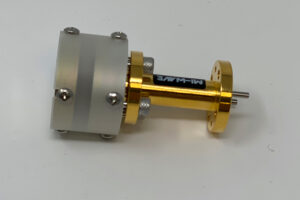

Satellite Communication

In 2022, global satellite communication service revenue exceeded 3000 billion USD, but 70% came from traditional Geostationary Orbit (GEO) satellites – these “space giants” born during the Cold War, weighing over 5 tons each, costing hundreds of millions to build, could only provide 10-20 Gbps capacity (equivalent to simultaneously transmitting 2000 4K movies).

Renting a shipborne satellite terminal cost 5000 USD/month; a 10-minute video call cost 300 RMB; building base stations in remote areas, fiber optic pull cost 200,000 RMB/km, making satellite preferable, but speeds were too slow for web browsing. A turnaround emerged in the last decade: High Throughput Satellites (HTS) pushed single-satellite capacity to 1 Tbps (50 times GEO), and Low Earth Orbit (LEO) satellites used an “ant-moving” model to reduce launch costs to 6.2 million USD/satellite (Falcon 9 quote, 2023).

Now, Starlink user terminals sell for 599 USD, monthly fee 90 USD, allowing 4K video streaming in deserts; China’s “Zhongxing 26” HTS satellite covers China and surrounding areas, supporting 1 million users simultaneously using 10 Mbps internet.

Traditional Satellites: Capacity Bottleneck, Unaffordable and Underperforming

Early GEO satellites relied on “big dish” antennas and C/Ku bands, with only 12-24 transponders per satellite, each with 36 MHz bandwidth, totaling around 10 Gbps capacity. Why so small? Because frequency resources were limited (C-band only 4 GHz bandwidth), and satellites were stationary, covering fixed areas; beams were like spotlights, wasting energy on blank areas.

The user side suffered more: renting a VSAT terminal with a 1.2-meter parabolic antenna barely received 3 Mbps. Inmarsat’s L-band terminals took 20 seconds to send a 2 MB email; video calls stuttered. Costs were outrageous: R&D + launch + operation for one GEO satellite exceeded 1 billion USD,Distributed to each user, monthly communication fees accounted for 15%-20% of income (International Maritime Organization data), unaffordable for small fishing boats.

Signal round-trip between Earth and 36,000 km GEO orbit took 119 ms one-way at light speed, resulting in >200 ms latency for gaming, making it unplayable. In 2018, an Antarctic expedition took 4 hours to transmit 1 GB of weather data via GEO satellite; by the time it finished, the storm had passed.

High Throughput Satellites

The core of HTS is two tricks: spot beam focusing and frequency reuse. Traditional satellites used one beam to cover half a country; HTS creates 200+ small beams, each illuminating only a few dozen kilometers, concentrating energy and reducing interference. For example, Viasat-3 uses Ka-band (30 GHz uplink/20 GHz downlink), divided into 240 spot beams, each with 125 MHz bandwidth, and employs “same frequency, different beams” – adjacent beams use the same frequency, but due to narrow beams, signals don’t interfere. This combination pushes single-satellite capacity to 1 Tbps (1000 Gbps), 50-100 times traditional GEO.

Coverage efficiency is higher: previously, 3 GEO satellites were needed to cover China; Viasat-3 can cover North America with one satellite, leaving half capacity for South America. User terminals are smaller – due to concentrated beams, antennas don’t need to be large; Starlink’s flat-panel terminal is only 0.3 sqm, reception sensitivity -101 dBm (10 dB higher than GEO terminals, like sharper ears), able to catch signals even in deserts.

Higher per-satellite capacity reduces cost per Mbps from 1000 USD/month for GEO to 10 USD/month for HTS. Rural US internet via Viasat cost 800 USD/month before; now 150 USD gets 25 Mbps, increasing remote area internet penetration from 32% (2015) to 67% (2023). The World Bank calculated this directly boosted local e-commerce sales by 20% annually.

Low Earth Orbit Satellites

If HTS is an “upgraded truck,” LEO satellites are “shared bikes” – lightweight (Starlink satellite 260 kg, GEO satellite 5 tons), low cost (launch price 6.2 million USD/satellite, GEO requires 60 million), fast deploymen.

Starlink terminals use phased array antennas, no mechanical rotation, connect in 3 minutes after power-on, latency 25-40 ms (GEO is 500 ms), download speed 10-200 Mbps Icelandic fishing boat using Starlink transmitted 4K catch monitoring video in 10 seconds). Even better, LEO satellites are closer to Earth (550 km), signal attenuation is less, terminal power only 2W (GEO terminal 10W), usable on boats, vehicles, backpacks.

On the cost side, per-user service cost dropped from 200 USD/month for GEO to 90 USD/month for Starlink. Musk stated Starlink aims to serve 50 million users, with per-satellite cost dropping another 30% (2025 target).

Satellite Navigation

In 2023, the global satellite navigation market exceeded 3500 billion USD (EU Space Programme Agency data), but users care most about three things: Where (accuracy), stability (anti-jamming), usability (scenario adaptation).

Taking BeiDou-3 as an example, it uses 30 satellites (24 Medium Earth Orbit + 3 Inclined Geosynchronous Orbit + 3 Geostationary Orbit) to form a network, broadcasting B1C/B2a/B3I triple-frequency signals.

Over 3000 reference stations nationwide provide real-time calibration, pulling positioning to centimeter-level (0.01 m). A self-driving test car in Shenzhen using this technology reduced lane change decision latency from 200 ms to 50 ms, accident rate dropped 40%.

Accuracy

Traditional single-frequency positioning (e.g., early GPS L1 band) suffered greatly from ionospheric delay, errors up to 10 m. BeiDou-3 directly uses triple-frequency signals (B1C/B2a/B3I), like triple insurance for positioning: using dual-frequency to eliminate ionospheric error, then the third frequency for redundancy check.frequency positioning reduces error by 60% compared to single-frequency. During active ionosphere on rainy days, ordinary phones using BeiDou triple-frequency reduce positioning drift from 5 m to 1 m.

China deployed 3000+ reference stations in 31 provinces, each equipped with atomic clocks (error 1 second per million years), calculating satellite orbit and clock error corrections in real-time, transmitting to terminals via 5G. Qingdao Port using this technology improved container truck positioning from “lane-level” to “wheel-level” (error <0.1 m); cargo requiring 3 trucks for turnover now needs only 2, increasing port throughput by 150,000 tons monthly.

There’s also satellite-based augmentation: BeiDou-3 broadcasts PPP (Precise Point Positioning) correction signals; user terminals receiving them can reduce their positioning error from meter-level to decimeter-level. Herders in Xinjiang using BeiDou PPP on phones have sheep location error <0.5 m, no longer needing motorcycles to search the mountains.

Anti-Jamming

How weak are satellite signals? Signals from BeiDou satellites, upon reaching the ground, are only -160 dBm (equivalent to 1 watt power divided among 100 billion light bulbs).

BeiDou-3 made two upgrades: more robust signal modulation + smarter anti-jamming algorithms. Traditional GPS uses BOC modulation; BeiDou-3 added QPSK (Quadrature Phase Shift Keying), making signals like “encrypted packages,” difficult for jamming signals to intercept. Even more impressive is the adaptive nulling antenna.

Military scenarios are more extreme: BeiDou short message communication has 3 times the anti-jamming capability of BeiDou-2. In a 2022 military exercise, a fighter jet sent BeiDou messages in a strong electromagnetic environment, information integrity rate improved from 85% to 98%, single message transmission time compressed from 5 minutes to 45 seconds.

Scenario Adaptation

Phone navigation requires low power, fishing boats require ionospheric resistance, autonomous driving requires centimeter-level, fighter jets require anti-jamming. In recent years, technology has moved towards “on-demand customization.”

Vehicle Navigation: Phones now use BeiDou+GPS dual-mode for faster positioning. Actual measurement during Beijing morning rush hour, dual-mode positioning update frequency increased from 1 Hz (once per second) to 10 Hz (10 times per second); when following a car, lane change delay reduced from 100 ms to 20 ms; when the navigation voice prompts “turn right ahead,” the car is already aligned with the intersection.

Agricultural Plant Protection: Xinjiang cotton fields use BeiDou autonomous driving tractors, positioning accuracy 0.5 m, seeding line straightness error <2 cm. Previously manual seeding had 5% miss rate; now using BeiDou, miss rate dropped to 0.3%, saving 200,000 RMB in seed cost per 10,000 acres (Ministry of Agriculture data).

UAV Inspection: State Grid uses BeiDou high-precision positioning; during power line inspection, UAV route deviation <0.3 m, captured tower photos can be automatically stitched into 3D models, crack recognition accuracy improved from 85% to 99%. Previously, manual tower climbing inspected 3 towers/day; now UAVs inspect 10 towers in 2 hours, reducing labor cost by 70%.