Horn Antenna Gain Calculation Guide | Formula, Aperture Area, Efficiency

Horn antenna gain is determined by the aperture area, operating wavelength, and efficiency (typically taken as 0.6).

The calculation formula is: 4π multiplied by the area multiplied by the efficiency, divided by the square of the wavelength.

A larger aperture area or a shorter wavelength results in higher gain, which significantly enhances the directional transmission capability of the signal.

The Fundamental Formula

The linear gain of a horn antenna follows the equation: G = (12.57 * A * e) / (L^2).

Where A represents the physical aperture area (square meters), e is the aperture efficiency (typically valued between 0.50 and 0.80), and L is the operating wavelength (meters).

At a frequency of 10 GHz, a 0.03-meter wavelength combined with a standard efficiency constant of 0.51 and an aperture area of 100 square centimeters produces a linear gain of approximately 71.2, which is 18.5 dBi.

Quantifying Efficiency Loss

For a standard pyramidal horn, when the E-plane aperture size and the horn length meet a specific ratio, the phase lag at the edges is usually controlled between 90 and 120 degrees.

If this phase difference exceeds 0.25 wavelengths, gain loss increases rapidly, leading to a significant reduction in effective area.

Experimental data shows that in a 10 GHz X-band environment, a horn with a length of 20 cm may see its phase error loss surge from 0.8 dB to over 1.5 dB if its aperture height is increased by 20%.

This loss is known in engineering calculations as the Phase Error Factor, which is the primary physical constraint preventing the infinite increase of high-gain antenna sizes.

Since rectangular waveguides primarily transmit the TE10 mode, the electric field at the H-plane aperture exhibits a distinct cosine distribution—meaning energy is strongest at the center and gradually decays to zero at the side walls.

While this natural energy taper helps suppress sidelobe levels (keeping them below -13 dB), it also causes a decrease in physical aperture utilization.

In an ideal uniform distribution, the amplitude efficiency can reach 100%, but in actual H-plane distributions, this ratio typically drops to about 81%.

If the uniform distribution of the E-plane is combined with the cosine distribution of the H-plane, the theoretical maximum efficiency is only about 81% (excluding phase errors).

In practical applications, designers often accept even lower amplitude utilization to balance beamwidth and gain.

In microwave measurement manuals, this power loss due to uneven electric field distribution is usually quantified as a fixed drop of approximately -0.9 dB.

For precisely calibrated standard antennas, this value must be accurately calculated by integrating the electric field intensity.

Combining phase error with amplitude distribution results in the engineering standard efficiency constant of 0.51.

This value is defined for “optimum gain horns,” where aperture dimensions are adjusted to maximize gain for a given horn length.

In this state, the E-plane phase difference parameter (s) is approximately 0.25, and the H-plane phase difference parameter (t) is approximately 0.375.

Under these conditions, the efficiency reduction due to phase error is about 0.8, while the amplitude distribution efficiency remains around 0.81.

Multiplying these and subtracting minor conduction losses results in a total efficiency stabilized near 51%.

In Ku-band (12.4 GHz to 18 GHz) measurements, the aperture efficiency of aluminum standard horns generally maintains between 50% and 55%, rarely exceeding 60% unless special flared or corrugated structures are used to correct the wavefront phase.

This physical compromise ensures stable radiation characteristics across a wide frequency band, but it also dictates that the relationship between linear gain (G) and physical area (A) always includes a fixed difference of approximately 3 dB.

In millimeter-wave bands, such as the Ka-band above 30 GHz, the skin effect on the internal walls of the horn becomes significant, and rough metal surfaces increase ohmic losses.

According to IEEE 149 standard test protocols, the conduction loss of an unpolished aluminum horn at 40 GHz can reach 0.15 dB to 0.2 dB.

While negligible at lower frequencies, this directly reduces the final dBi value in precision link budgets.

Additionally, structural deviations in the transition between the horn throat and the feed waveguide can cause an increase in the Voltage Standing Wave Ratio (VSWR).

An antenna with a VSWR of 1.2 has a return loss of approximately 0.035 dB, meaning 0.8% of the power is reflected back to the source.

When the operating frequency deviates from the design center frequency, the change in wavelength alters the values of the phase error parameters (s and t), causing efficiency to fluctuate within the band.

Across a 1.5:1 frequency coverage range, the efficiency fluctuation typically jumps between 45% and 55%.

For example, in a horn operating at 18 GHz, if the frequency rises to 26 GHz, while the physical area remains unchanged and the shorter wavelength favors a gain increase, the sharp increase in phase error will cause efficiency to drop rapidly below 40%, resulting in an actual gain growth far below the expectation based on the square of the frequency ratio.

Therefore, when writing link analysis reports, a dynamic efficiency model based on frequency changes must be used instead of simply substituting the static constant of 0.51, ensuring that the predicted signal strength error remains within a safe margin of 0.5 dB across the entire operating bandwidth.

Wavelength and Frequency Comparison

In free-space electromagnetic propagation, frequency and wavelength share a strict inverse relationship, mediated by the speed of light constant (299,792,458 m/s).

When the design frequency is increased from 8.2 GHz to 12.4 GHz, the corresponding WR-90 band wavelength decreases from 36.5 mm to 24.2 mm.

In the gain formula, since the wavelength is in the denominator and squared, any slight decrease in wavelength triggers an exponential rise in linear gain (G).

For a horn with a fixed aperture of 10 cm x 10 cm, the wavelength at 10 GHz is 3 cm, yielding a theoretical linear gain of approximately 71.2;

However, when the frequency doubles to 20 GHz, the wavelength shrinks to 1.5 cm, and the same physical area produces a linear gain jump to approximately 284.8.

This growth characteristic based on the square of the frequency is expressed on a decibel scale as an increase of approximately 6.02 dBi every time the frequency doubles.

The table below shows the wavelength and gain evolution data for different standard frequency bands, assuming a fixed physical area of 0.01 square meters and an aperture efficiency of 0.51:

Band Name	Center Freq (GHz)	Wavelength (mm)	Linear Gain (G)	Gain (dBi)	Beamwidth (E-plane/deg)
L Band	1.5	200.0	0.16	-7.94	102.0
S Band	3.0	100.0	0.64	-1.94	51.0
C Band	6.0	50.0	2.56	4.08	25.5
X Band	10.0	30.0	71.2	18.53	15.3
Ku Band	15.0	20.0	160.3	22.05	10.2
K Band	20.0	15.0	285.0	24.55	7.7
Ka Band	35.0	8.57	872.4	29.41	4.4
V Band	60.0	5.0	2564.0	34.09	2.6
W Band	94.0	3.19	6289.0	37.99	1.6

In the IEEE 149 standard antenna test procedure, frequency changes not only alter the absolute gain value but also affect the utilization rate of the effective aperture via the phase error factor.

As frequency rises, even though the smaller wavelength (L) favors gain enhancement, the phase distribution formed at the horn aperture becomes sharper.

If the axial length of the horn is fixed, rising frequency causes the phase error parameters (s and t) to increase, leading aperture efficiency to slide from 55% at lower frequencies to 45% or lower at higher frequencies.

Within the 12.4 to 18 GHz range covered by WR-62 waveguides, the measured efficiency of a standard gain horn might reach 0.53 at the lower frequency point but drop to 0.49 at the higher end due to accumulated phase difference.

This dynamic fluctuation in efficiency offsets part of the gain increase brought by wavelength reduction, making the actual gain-vs-frequency curve slightly lower than the theoretical 20 log growth slope.

In engineering plots, this phenomenon is quantified as gain flatness error, usually maintained within a fluctuation range of 1.5 dB to 2.0 dB across the entire waveguide bandwidth.

In low-frequency applications at 1 GHz, a 300 mm wavelength means a 1 mm processing error only generates a 1.2-degree phase deviation, which hardly affects the final gain.

However, in the 94 GHz millimeter-wave band, a 3.19 mm wavelength means that same 1 mm error produces over 110 degrees of phase distortion, causing severe radiation pattern deformation and a catastrophic drop in gain.

NIST (National Institute of Standards and Technology) calibration reports mention that for horns operating above 40 GHz, the flatness of the aperture edges and the roughness of the internal plating must be controlled within one-fiftieth of a wavelength (below 0.06 mm) to ensure consistency between measured gain and calculated values.

Waveguide Model	Freq Range (GHz)	Wavelength Range (mm)	Typ. Horn Length (mm)	Expected Gain (dBi)
WR-90	8.2 – 12.4	36.5 – 24.2	200 – 250	15 – 22
WR-62	12.4 – 18.0	24.2 – 16.7	150 – 180	16 – 23
WR-42	18.0 – 26.5	16.7 – 11.3	100 – 130	18 – 24
WR-28	26.5 – 40.0	11.3 – 7.5	60 – 90	20 – 25

Near 60 GHz, there is a strong absorption peak caused by oxygen molecules, with attenuation rates reaching around 15 dB/km.

This means that even if an antenna gains over 30 dBi through wavelength reduction, the signal strength received in an actual far-field link remains limited by frequency-dependent atmospheric constraints.

In contrast, in the 10 GHz or 35 GHz atmospheric window bands, the gain advantages brought by wavelength can be fully preserved in the link margin.

Measurement data shows that at the same power output, a Ka-band horn system provides an Effective Isotropic Radiated Power (EIRP) approximately 11 dB higher than an X-band system due to its shorter wavelength and higher gain, but its beamwidth narrows by nearly 70%, placing much higher requirements on alignment accuracy.

Numerical Conversion Steps

After completing the preliminary calculation of the basic physical formula G = (12.57 * A * e) / (L^2), the resulting value is a dimensionless pure number representing the power enhancement ratio.

To facilitate cascaded calculations in complex microwave links, this must be converted into a decibel value relative to an isotropic radiator (dBi).

The conversion process uses the standard logarithmic model: 10 * log10(G). It must be clarified that gain is a manifestation of power ratios; therefore, the coefficient 10 must be used instead of the voltage ratio coefficient 20.

If the linear gain (G) calculation result is 100, the result after logarithmic operation is exactly 20.00 dBi.

In actual engineering, G values often carry complex floating-point decimals. For instance, in a WR-90 waveguide experiment, an 18.25 cm long horn at 10 GHz might have a calculated linear gain of 66.83, which corresponds to approximately 18.25 dBi.

Retaining at least two decimal places when processing these figures is a fundamental requirement to ensure that the total system error is controlled within 0.5 dB.

The table below lists the precise correspondence between common linear gain multiples and decibel values (dBi), along with their physical performance in power distribution:

Linear Gain (G)	Gain (dBi)	Power Enhancement Description	Typical Antenna Type Reference
1.00	0.00	No enhancement, same as point source	Ideal Isotropic Radiator
1.64	2.15	1.64x power concentration	Free-space half-wave dipole
10.00	10.00	10x power concentration	Small wide-beam waveguide horn
31.62	15.00	~31.6x power concentration	Medium gain standard gain horn
100.00	20.00	100x power concentration	Lab-standard calibration horn
316.23	25.00	~316x power concentration	High-gain narrow-beam pyramidal horn
1000.00	30.00	1000x power concentration	Precision long-range detection horn

For low-gain antennas below 10 dBi, a fluctuation of 0.5 in the linear value only produces a ripple of about 0.2 dB;

However, for high-gain systems above 25 dBi, a deviation of 10 in the linear value can trigger a calculation offset exceeding 0.15 dB.

In test reports for satellite communication ground station feeds, the conversion steps must include negative compensation for connector loss and internal return loss.

For example, if the theoretical calculation yields 22.45 dBi, but there is 0.12 dB of impedance mismatch loss and 0.05 dB of ohmic loss on the metal surface, the final value entered into the system parameters should be corrected to 22.28 dBi.

This subtle numerical correction corresponds to about 4% of actual power loss, which can cause the signal-to-noise ratio at the receiver to drop by about 0.3 dB in long-distance communications, thereby affecting Bit Error Rate (BER) performance.

The following is a data processing checklist that must be strictly followed during the numerical conversion process:

• Input Verification: Ensure that the linear gain (G) substituted into the logarithmic formula is the effective value considering aperture efficiency (e), rather than just the geometric area ratio.
• Constant Unification: When calculating wavelength (L) using the speed of light, 299,792,458 m/s should be used uniformly to avoid the 0.07% frequency drift error caused by using 300,000,000 m/s.
• Unit Consistency: When calculating A / L^2, the aperture area (A) must be in square meters, and the wavelength (L) must be in meters; otherwise, the linear value will have a 10,000-fold error, causing the decibel value to deviate by 40 dB.
• Significant Figure Truncation: Engineering calculations suggest retaining four significant figures before the logarithmic operation and two decimal places for the resulting decibel value to match the measurement precision of a VNA.

When the frequency is increased from 10 GHz to 20 GHz, the wavelength is halved, and the linear gain (G) jumps from 100 to 400—a fourfold increase in value;

However, on a decibel scale, this change is expressed only as an increase from 20 dBi to 26.02 dBi (an increase of 6.02 dB).

This logarithmic compression effect makes decibel values more suitable for describing perceived changes in signal strength.

NIST calibration specifications mention that in millimeter-wave bands (e.g., 60 GHz), where path loss is extremely high, any numerical conversion fluctuation below 0.05 dB can be amplified in the link budget.

Therefore, using high-order logarithmic algorithms or specialized mathematical software for conversion, rather than manual log tables, is the standard procedure for modern microwave laboratories.

Decibel Difference (dB)	Linear Power Loss Ratio	Linear Power Gain Ratio	Power Change % Description
0.1	0.977	1.023	~2.3% slight fluctuation
0.5	0.891	1.122	~11% moderate change
1.0	0.794	1.259	~21% significant change
3.0	0.501	1.995	~50% doubling or halving
10.0	0.100	10.000	10-fold magnitude change

When handling asymmetric horn antennas (where E-plane and H-plane flare angles differ), the numerical conversion step must also introduce an additional correction parameter to account for phase center offsets caused by non-square apertures.

In this case, the calculation process usually involves finding the effective aperture gain for both planes individually, calculating the geometric mean, and then performing the 10 * log10 operation.

For a horn operating at 28 GHz with an aperture size of 40 mm x 30 mm, its measured linear gain is approximately 218.5, and the converted 23.39 dBi should be marked with a ±0.2 dB confidence interval on the calibration certificate.

Aperture Area

The physical area is directly measured from the length and width of the opening (rectangular) or the diameter (circular).

For example, a standard X-band horn (8.2 to 12.4 GHz) typically has a physical aperture area between 50 and 150 square centimeters.

Due to phase deviations and uneven amplitude distribution, the actual effective area is usually only 50% to 80% of the physical area.

At 10 GHz, with a 3 cm wavelength and a 100 cm² aperture at 0.7 efficiency, a gain of approximately 19.9 dB can be obtained.

Physical Dimension Measurement

A typical Ka-band (approx. 33 GHz) conical horn usually has its feed end connected to a WR-28 waveguide-to-circular waveguide adapter, where the internal diameter of the circular waveguide is approximately 7.1 mm.

To achieve high directivity, the aperture diameter might expand to between 50 mm and 80 mm. In actual machining, the flatness and circularity deviations of the horn’s inner walls must be controlled within 0.02 mm.

The physical area calculation is based on 3.14159 multiplied by the square of the radius.

At 35 GHz, where the wavelength is only 8.57 mm, a tiny 1 mm error in aperture diameter results in a 3% to 5% change in aperture area.

Furthermore, the axial length of the horn directly limits the flare angle, which is typically recommended to be between 15 and 20 degrees.

If the flare angle is too large, even though the physical aperture increases, the effective area utilization will drop below 0.4 due to phase irregularities.

In the structure of a pyramidal horn, the measurement of physical dimensions involves more complex four-sided expansion parameters.

Below are typical physical dimension measurement references for different gain requirements:

• 15 dBi Requirement: In the X-band, aperture dimensions are approx. 80 mm x 60 mm, axial length is approx. 120 mm, with a total physical envelope volume of about 432 cm³.
• 20 dBi Requirement: Aperture dimensions increase to 145 mm x 110 mm. To maintain phase consistency, the axial length must be stretched beyond 260 mm, with the physical volume surging to about 4147 cm³.
• 25 dBi Requirement: Aperture size typically reaches 280 mm x 210 mm, and axial length may exceed 600 mm, placing high demands on the mechanical strength of the mounting brackets.

When using aluminum alloy materials and CNC milling, wall thickness is usually set between 2 mm and 5 mm to ensure the horn does not deform under high temperature or vibration environments.

External physical dimensions are typically measured using electronic digital calipers, while complex internal cavity dimensions require multi-point sampling via a Coordinate Measuring Machine (CMM).

For corrugated horn antennas, the depth and width of the internal slots are also part of the physical measurement, with slot depth typically designed as one-quarter of the operating wavelength (approx. 0.25 * wavelength).

For example, at 12 GHz, the corrugated slot depth is about 6.25 mm and the slot width is about 2 mm.

These microscopic physical dimensions exist to force the electromagnetic waves into a more uniform amplitude distribution across the aperture plane.

When measuring aperture area, the space occupied by the flange must be considered.

Standard flanges like UG-39/U increase the physical footprint at the bottom of the antenna but do not count towards the electromagnetic aperture area.

In system integration plans, engineers must distinguish between the “Effective Electromagnetic Aperture” and the “Total Physical Outline.”

In high-frequency bands like the W-band (75-110 GHz), the wavelength shrinks to about 3 mm, making the surface roughness of the horn’s inner walls (typically required to be below 0.8 microns) a hidden cost in physical dimension control.

If the inner walls are not smooth enough, it is equivalent to changing the local physical propagation path, causing measured gain to be lower than theoretical values.

For sectoral horns, physical dimension measurement exhibits asymmetry.

An E-plane sectoral horn expands in only one plane; its aperture height might reach 200 mm while the width remains consistent with the waveguide at about 10 mm.

This special physical ratio produces a wide horizontal beam and a narrow vertical beam.

When measuring such antennas, the symmetry of the expansion angle is a focus of evaluation; if the offset of the left wall vs. the right wall relative to the center axis exceeds 0.5 degrees, the beam center will physically shift.

High-precision laser scanners can capture physical area data for every millimeter of the horn’s cross-section, allowing for precise simulation models to predict actual radiation efficiency.

All physical data is ultimately summarized in the design manual as the sole factual basis for subsequent installation, gain calibration, and link calculations.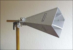

Gain Proportionality Laws

Since gain is inversely proportional to the square of the wavelength, if the aperture area is fixed at 100 cm², increasing the frequency from 10 GHz to 20 GHz will halve the wavelength.

According to the gain proportionality law, halving the wavelength causes the denominator to become one-fourth of its original value, thereby increasing the gain value by 6 dB.

This explains why in millimeter-wave bands (e.g., 60 GHz or 94 GHz), even extremely small physical horns can achieve gains comparable to huge parabolic antennas at lower frequencies.

For systems operating in the Ku-band (12 to 18 GHz), gain rises steadily at a slope of approximately 0.5 to 0.8 dB for every 1 GHz increase in frequency, assuming the aperture remains constant.

Operating Freq (GHz)	Wavelength (mm)	Assumed Aperture (m²)	Efficiency Coeff	Theo. Gain (dBi)
2.4 (S-band)	125.0	0.04	0.55	11.4
5.8 (C-band)	51.7	0.04	0.55	19.1
10.0 (X-band)	30.0	0.04	0.55	23.8
24.0 (K-band)	12.5	0.04	0.55	31.4
35.0 (Ka-band)	8.57	0.04	0.55	34.7
94.0 (W-band)	3.19	0.04	0.55	43.3

Ideally, physical area can be fully converted to effective area, but in reality, the expansion angle of the horn causes edge phase lag.

For a large-aperture horn with a short axial length, efficiency can be as low as 0.4. In this case, even with a large physical area, the measured gain will be lower than expected.

Typically, standard gain horns are designed with an efficiency stabilized around 0.5, allowing for linear gain growth without excessively large volumes.

When efficiency increases from 0.5 to 0.7, the gain increases by approximately 1.46 dB.

In actual engineering applications, the relationship between gain and size is also constrained by the Slant Length.

If pursuing high gains above 25 dB, simply increasing the aperture area is insufficient.

According to gain laws, every time the aperture diameter doubles, the axial length of the horn must increase fourfold to maintain phase error within limits.

This leads to high-gain horns often having a very slender shape.

For example, a 20 dBi X-band horn might be only 250 mm long, but to reach 30 dBi, the length could exceed 1.5 meters.

This non-linear growth in volume is due to the necessity of balancing phase distortion caused by area expansion.

In satellite ground station feed designs, this proportionality constraint often forces designers to use corrugated horns or dielectric loading techniques to simulate a larger effective aperture within a shorter physical length.

Target Gain (dBi)	Area Increase (Ref 10 dBi)	Expected Efficiency	Typ. Side Length (@ 10 GHz)	Phase Deviation Risk
10	1.0 (Base)	0.60 – 0.80	35 mm	Extremely Low
15	3.16	0.55 – 0.75	65 mm	Low
20	10.0	0.50 – 0.65	115 mm	Medium
25	31.6	0.45 – 0.55	210 mm	High
30	100.0	0.40 – 0.50	380 mm	Extremely High

According to the radar equation, for every 6 dB increase in antenna gain, the theoretical detection range of the radar can double, assuming other parameters remain constant.

Since the wavelength of a 77 GHz radar is only 3.9 mm, a compact 4 cm x 4 cm horn aperture can provide a gain of over 25 dBi.

When performing such high-frequency designs, the surface roughness of the aperture must be controlled within one-thirtieth of a wavelength; otherwise, the drop in efficiency caused by surface scattering will break the gain-to-area proportionality, causing actual performance at high frequencies to be much lower than predicted by mathematical models.

Due to the symmetry of conical structures in polar coordinates, their aperture efficiency is more stable over a wide frequency band than rectangular horns.

At an operating frequency of 30 GHz, a 20 mm diameter conical aperture gain is approx. 15.5 dBi. When the diameter increases to 40 mm, the gain jumps to about 21.5 dBi.

This 6 dB span again validates the physical logic that quadrupling the area (doubling the radius) corresponds to quadrupling the gain.

In ultra-wideband applications, gain presents an inclined curve as the frequency is scanned—the higher the frequency, the greater the gain. This tilt rate is a variable that must be offset in link budget balancing.

Aperture Shape Selection

A conical horn operating in the 30 GHz Ka-band typically has an aperture diameter between 45 mm and 60 mm, which, when paired with circular waveguide feeding, can achieve an axial ratio below 1 dB.

When calculating the area of a circular aperture, the numerical basis is 3.14159 multiplied by the square of the radius.

Although the theoretical gain of a circular aperture is equivalent to a rectangular one of the same area, its lateral beam distribution is more uniform, with sidelobe levels usually maintained between -18 dB and -22 dB—better than the -13 dB of a standard rectangular opening.

According to experimental data in microwave design manuals, when the half-flare angle of a conical horn is controlled at approximately 15 degrees, the phase consistency at the opening performs best, and the ratio of physical area converted into effective area can stabilize above 0.55.

Aperture Shape	Interface Standard	Typ. Size @ 12 GHz (mm)	Gain Potential	Polarization
Pyramidal	WR-75	115 x 90	Medium to High	Linear
Sectoral E-plane	WR-75	180 x 19	Low (Fan Beam)	Strongly Dir. Linear
Conical	20mm Circular	Diameter 85	Medium	Circular/Linear
Corrugated	18mm Circular	Diameter 110	Extremely High (0.8 eff)	Excl. Cross-pol

When system requirements for Sidelobe Level (SLL) are extremely strict, Corrugated Horns become the advanced selection for aperture shape.

While these horns appear conical on the outside, their inner walls are carved with ring-shaped slots approx. one-quarter wavelength deep.

At a frequency of 12 GHz, the slot depth is about 6.25 mm. These physical slots force the electromagnetic waves to exhibit a Gaussian distribution at the aperture plane.

Experimental data shows that the aperture efficiency of a corrugated horn can be increased from 0.5 for a standard horn to 0.75 or even 0.82.

In the same physical envelope volume, a corrugated shape can provide about 1.5 to 2 dB more gain than a smooth conical shape.

Furthermore, corrugated apertures have almost no significant sidelobe interference beyond -30 dB, which is critical for deep space exploration and high-precision weather radar.

In specific engineering dimension measurements, aperture shape selection is also linked to manufacturing costs and weight distribution.

Rectangular horns can be manufactured from four aluminum plates via welding or precision sheet metal bending, with thicknesses typically between 1.5 mm and 3 mm. A 15 dBi X-band horn can be kept under 500 grams.

In contrast, high-performance circular corrugated horns usually require CNC turning from solid aluminum blocks.

To ensure slot depth, the wall thickness often reaches over 8 mm, making them 3 to 5 times heavier than rectangular horns of equivalent gain.

In designs for UAV-borne radar or portable satellite terminals, this weight difference often determines the final physical layout.

For millimeter-wave bands above 60 GHz, where wavelengths shrink to below 5 mm, tiny deformations in aperture shape (e.g., 0.05 mm flatness deviation) lead to radiation pattern distortion.

Therefore, in W-band (75-110 GHz) designs, circular apertures are favored for their ease of maintaining machining concentricity.

If a system requires 120-degree coverage in the horizontal direction and only 10 degrees in the vertical direction, engineers use extremely flat sectoral apertures.

Although the physical area of such apertures seems large due to extreme elongation in one dimension, since the height might even be smaller than the waveguide wavelength, the gain is usually not very high, fluctuating between 8 and 12 dBi.

When measuring such antennas, one must focus on quantifying the position of the phase center, as it often shifts by more than 10 mm as frequency changes in flat apertures.

The IEEE standard antenna selection guide states: “Every geometric discontinuity in the aperture shape introduces additional reactive components.”

Thus, in transition zones from rectangular to circular, smooth transition sections of at least two wavelengths in length must be designed to ensure impedance matching and maintain a low VSWR below 1.1.

From the perspective of antenna array integration, aperture shape determines the packing density of array elements.

Rectangular apertures, having flat physical edges, allow for seamless and compact tiling.

In phased array radar feed arrays, this geometric feature allows more antenna units to be packed into a limited aperture, thereby enhancing the total Effective Isotropic Radiated Power (EIRP).

Conical horns inevitably leave triangular physical gaps when tiled, leading to a drop of about 10% to 15% in the utilization of total physical area.

However, in high-performance reflector antennas (e.g., Ku-band receiving stations with diameters over 3 meters), the symmetric beam provided by conical corrugated horns ensures that the edge illumination level of the reflector is uniformly distributed around -10 dB, thereby minimizing the spillover loss of the entire antenna system.

Aperture Efficiency

For standard pyramidal horns, this ratio is typically between 0.45 and 0.55, while corrugated horns can reach 0.7 to 0.8.

If efficiency drops from 0.8 to 0.4, gain will decrease by approximately 3 dB.

This metric is influenced by both the non-uniformity of the aperture field distribution and the wavefront phase difference.

In frequency bands above 10 GHz, the utilization of the physical aperture is directly limited by the horn’s axial length and flare angle.

Fundamentals of Efficiency

From an electromagnetic theory perspective, during the process of converting electromagnetic waves from a waveguide to free space, the actual capacity to capture or transmit energy is always lower than the ideal state suggested by the geometric cross-section due to uneven aperture field distribution and phase deviations.

In engineering calculations, this metric is defined as the ratio between the effective area and the physical area.

For a standard gain horn, typical efficiency values fall between 0.50 and 0.52.

If an X-band horn at 10 GHz has an aperture size of 10 cm x 8 cm, its physical area is 80 cm², but in actual link estimation, only about 40 to 41 cm² of that area truly contributes to gain.

Aperture efficiency is typically broken down into the following independent components for quantitative analysis during the design phase:

• Illumination Component: In rectangular horns, the basic propagation mode is TE10. The electric field of this mode is distributed sinusoidally across the aperture width—highest at the center and nearly zero at the edges. This uneven distribution means that even without phase error, aperture utilization can only reach a maximum of about 0.81.
• Phase Error Component: Because the straight path from the waveguide feed to the center of the aperture is shorter than the diagonal path to the edges, the wavefront at the aperture is curved rather than flat. This phase inconsistency causes destructive interference in the far field, significantly reducing main-lobe intensity.
• Edge Diffraction Loss: When electromagnetic waves reach the metal edges of the horn, some energy is diffracted. This energy cannot be concentrated into the intended beam, resulting in an efficiency reduction of about 1% to 3%.
• Cross-Polarization Component: If the inner walls are not smooth or the design is unbalanced, some vertical polarization converts to horizontal polarization, which cannot be extracted by a co-polarized receiving antenna.

According to Balanis antenna theory, when the E-plane phase difference is controlled within 0.25 wavelengths and the H-plane phase difference within 0.375 wavelengths, horn gain peaks.

At this point, the calculated comprehensive aperture efficiency is precisely around 51.1%.

In a fixed physical aperture scenario, blindly increasing the horn length improves phase but increases volume and weight;

Conversely, shortening the length and increasing the flare angle causes phase error to accumulate rapidly, dropping efficiency below 0.3 and even causing beam splitting.

Antenna Parameter	Impact Trend	Data Ref (12 GHz)
Inc. Axial Length	Phase flatness up, efficiency up	+20% length = +5% eff.
Inc. Flare Angle	Phase error up (sq.), efficiency down	Angle >40° = eff. <40%
Corrugated Walls	Symmetric distribution, edge currents suppressed	Eff. can rise from 51% to >75%
Rising Frequency	Surface precision impact increases	0.1mm error = 3% eff. fluctuation (@Ka)

The calculation of wavefront phase difference (s) typically depends on the horn’s geometric slant distance (l) and half-aperture width (a), expressed as s = a^2 / (2 * l).

In Ku-band or higher satellite communication ground stations, engineering personnel often install dielectric lenses at the horn aperture to compensate for this phase difference.

Horns with lenses can have aperture efficiencies boosted from a standard 0.5 to 0.85 or even over 0.9.

While this increases system complexity and weight, it allows gain to increase by about 2.5 dB without changing physical aperture size.

Due to circular symmetry, its illumination efficiency in the TE11 mode is slightly higher than that of rectangular horns, but phase error impacts remain. In unoptimized cases, typical efficiency is about 0.522.

In applications like radio astronomy or deep space exploration, Corrugated Horns are used for purer polarization performance.

These force the electric field to zero at all edges, creating a highly symmetric HE11 hybrid mode, stabilizing aperture efficiency between 70% and 80%.

“The ratio of effective area Ae to physical area Ap directly defines the upper limit of the system’s capacity to capture free-space energy.”

In actual link budget formulas, Gain (G) calculation is expressed as G = (4 * PI * Ae) / lambda^2, where Ae = efficiency * Ap.

If an engineer designing a 28 GHz 5G base station antenna ignores the frequency-dependent fluctuation of efficiency and calculates based only on physical area, the predicted coverage will be 30% to 40% larger than actual test results, because surface roughness and machining tolerances further dilute aperture efficiency at high frequencies.

In millimeter-wave designs above 40 GHz, the impact of tiny physical deformations on aperture efficiency exhibits non-linear growth.

For a standard horn with a nominal gain of 20 dBi, if thermal deformation from uneven wall thickness occurs at the opening, the phase center will shift. This not only lowers gain but also raises sidelobe levels by more than 5 dB.

Therefore, in the aerospace field, calibration for such horns usually includes physical efficiency measurements, back-calculating actual efficiency by comparing the received level against a known Standard Gain Horn in an anechoic chamber.

To further enhance efficiency, modern computational electromagnetics software often uses genetic algorithms to optimize the horn’s wall envelope into non-linear profiles, forming “beam-shaped horns.”

These horns are no longer simple linear expansions but have curved transition profiles, reducing mode conversion loss and distributing energy more uniformly across the aperture.

Experimental data shows that these profile-optimized horns achieve aperture efficiencies approx. 15% higher than traditional linear flare horns while maintaining compact structures.

Performance of Different Models

Conical horns exhibit different radiation characteristics, formed by the gradual expansion of a circular waveguide, primarily transmitting the TE11 mode.

Due to the symmetry of the circular structure, these antennas have a natural advantage in handling circularly polarized signals.

Without additional optimization, the typical aperture efficiency of a conical horn is approximately 52.2%, slightly higher than that of a pyramidal horn.

This efficiency boost comes from the electric field distribution in circular waveguide modes being closer to the aperture center, thereby reducing edge leakage.

However, E-plane and H-plane patterns for standard conical horns still show significant differences, and sidelobe levels are usually around -18 dB.

In satellite link feed designs, simple conical horns are often limited by high cross-polarization levels (typically around -20 dB). To improve this, the flare angle is often limited to within 10 degrees to obtain better phase center stability.

Data shows that a conical horn with an aperture diameter of 3 wavelengths has a main-lobe 3 dB width of about 20 degrees, providing good directivity for point-to-point microwave communication.

E-plane sectoral horns expand in the vertical direction, producing a beam that is wide horizontally and narrow vertically; H-plane sectoral horns do the opposite.

The efficiency of these antennas fluctuates greatly, usually between 0.40 and 0.60.

Since expansion occurs in only one plane while the other remains at the original waveguide dimension, phase error exists only in the expanded plane.

In practical applications like fan-beam scanning for ground navigation radar, H-plane sectoral horns are widely used because they provide narrower azimuthal resolution.

Test data indicates that when the H-plane flare angle increases beyond 30 degrees, aperture efficiency drops rapidly below 45% unless length is increased proportionally.

Corrugated horns represent the high-performance technical standard for horn antennas, with ring-shaped grooves machined into the inner walls at a depth of approx. one-quarter wavelength.

These structures change the boundary conditions, causing E-plane and H-plane conditions to converge, producing highly symmetric HE11 hybrid modes.

A significant feature of this mode is that the electric field almost completely vanishes at the aperture edges, eliminating edge diffraction loss.

The aperture efficiency of corrugated horns typically reaches 0.75 to 0.82, and in high-performance satellite ground station feeds, this can stabilize above 0.8.

These antennas have extremely low sidelobe levels, usually less than -30 dB, and cross-polarization isolation can be better than -35 dB.

Although the manufacturing process is complex and the weight is high, the resulting gain increase of over 2 dB and extremely high signal purity make it the preferred model for deep space exploration and radio astronomy.

Model Name	Typ. Gain Range (dBi)	Aperture Eff. (Typ.)	Sidelobe Level (dB)	Phase Center Stability
Standard Pyramidal	15 – 25	0.51	-13	Medium
Standard Conical	12 – 20	0.52	-18	Good
E-plane Sectoral	10 – 18	0.45	-12	Poor (Asymmetric)
High-Perf. Corrugated	18 – 30	0.78	-32	Excellent
Stepped Transform	15 – 22	0.65	-22	Good

Stepped transform horns or multi-mode horns excite higher-order modes (such as the TM11 mode) by setting abrupt steps inside the horn.

By precisely controlling the amplitude and phase ratios between the fundamental and higher-order modes, the field distribution on the aperture can be artificially smoothed.

This method extends energy that was originally concentrated at the center towards the edges, thereby increasing aperture utilization.

Measured data proves that this multi-mode compensation technique can increase the efficiency of standard conical horns from 52% to around 65%.

In X-band experiments, a horn corrected with the TM11 mode showed a gain about 1.2 dB higher than a standard horn at 9.5 GHz.

Addressing the needs of modern compact equipment, Profiled Horns replace traditional linear flare angles with non-linear wall envelopes.

This curved design achieves a smooth transition of modes inside the horn, significantly reducing reflection loss from mode conversion.

Their length is typically 30% to 50% shorter than standard horns of the same gain, yet aperture efficiency can be maintained at around 0.70.

In millimeter-wave bands like 60 GHz, where atmospheric attenuation is severe, these high-efficiency, short-length horns are vital for integration into miniaturized transceiver front-ends.

Experimental data shows that a 60 GHz profiled horn only 2 cm long can still provide 18 dBi of gain, with efficiency fluctuations below 5% across the entire band.

Frequency Band	Model Example	Physical Aperture (mm)	Measured Gain (dBi)	Estimated Eff.	Cross-pol (dB)
C-band (5 GHz)	Pyramidal	240 * 180	19.5	0.51	-25
Ku-band (12 GHz)	Conical	80 (Diam.)	18.2	0.53	-22
Ka-band (30 GHz)	Corrugated	45 (Diam.)	21.8	0.79	-38
V-band (60 GHz)	Profiled Opt.	15 * 12	17.5	0.68	-28

For models above 40 GHz, the surface roughness of the inner walls directly introduces additional scattering loss, leading to decreased efficiency.

For example, in the Ka-band, if the inner wall roughness increases from 1 micron to 5 microns, aperture efficiency may drop an additional 2% to 4%.

Therefore, high-performance corrugated or profiled horns are often manufactured using electroforming to ensure microscopic smoothness and geometric precision.

Interference Factors

In the design and gain evaluation of horn antennas, factors interfering with gain performance primarily stem from phase deviations caused by geometric structure, non-uniformity of aperture field distribution, physical machining precision, and electromagnetic properties of materials.

Looking at the physical process of electromagnetic wave propagation inside the horn, the wavefront diffusing from the waveguide feed is not an ideal plane wave but a curved spherical wave.

This geometric path difference is the main physical mechanism interfering with gain growth.

The path length for electromagnetic waves reaching the aperture center along the axis is significantly shorter than the diagonal path to the aperture edges.

This phase excess caused by path difference accumulates quadratically as the flare angle increases.

In 12 GHz Ku-band applications, if the phase difference between the aperture edge and center reaches 0.125 wavelengths, gain loss is typically around 0.1 dB; however, once the phase difference expands to 0.5 wavelengths, gain not only stops growing but severe beam distortion and approximately 3 dB of attenuation occur.

In standard rectangular horns, electric field intensity follows the TE10 mode’s sine distribution law in the H-plane.

Electric field intensity near the edges approaches zero, resulting in the physical edges contributing far less to far-field radiation than the center area.

This non-uniformity in illumination caused by mode characteristics limits theoretical maximum efficiency to about 81%.

• Geometric Phase Error: Limited by finite axial length, wavefront curvature prevents phase synchronization across the aperture.
• Amplitude Taper: Waveguide modes dictate lower energy at aperture edges, preventing full utilization of the physical area.
• Impedance Mismatch: Abrupt transitions between the waveguide and horn, as well as boundary reflections between the horn opening and free space, generate standing waves.
• Surface Loss: Internal wall conductivity and roughness cause significant ohmic losses in millimeter-wave bands.
• Structural Tolerances: Throat misalignment or insufficient wall flatness excites parasitic modes, interfering with polarization purity.

A well-designed horn antenna should typically have a Voltage Standing Wave Ratio (VSWR) below 1.15:1.

If poor throat design causes the VSWR to rise to 1.5:1, reflection loss reaches about 0.17 dB. While seemingly small, in high-precision link budgets, this energy uncertainty interferes with the accurate determination of effective area.

Furthermore, in high-frequency bands above 30 GHz, the microscopic structure of material surfaces becomes a non-negligible interference component.

“In high-frequency electromagnetic fields, current flows only within the skin depth of the metal surface; the machining roughness of the inner walls directly determines the magnitude of conduction loss.”

In the Ka-band (approx. 35 GHz), skin depth is only about 0.35 microns.

If the average roughness of the inner walls of an aluminum or copper horn exceeds 1 micron, electromagnetic waves generate additional scattering and heat loss during reflection, causing gain to be 0.2 to 0.5 dB lower than theoretical expectations.

Interference Component	Physical Source	Data Ref (20 GHz)	Impact on Gain
Phase Lag	Excessive Flare Angle	Edge Phase Diff > 90°	Gain drops > 1.5 dB
Amplitude Dist.	TE10 Mode Props	Edge intensity 10% of center	Eff. limited to 50-60%
Return Loss	Impedance Mismatch	VSWR = 1.25	~0.05 dB power loss
Ohmic Loss	Surface Conductivity	Roughness 2 microns	~0.15 dB radiation eff. drop
Cross-polarization	Mode Impurity	Isolation < 25 dB	Lowered co-pol reception eff.

For aluminum horn antennas, the thermal expansion coefficient is approximately 23 x 10⁻⁶ per degree Celsius. When the operating environment temperature difference reaches 80°C, a large X-band horn’s aperture might generate nearly 0.5 mm of deformation.

This impact is negligible at 10 GHz, but in the 60 GHz V-band, such size drift causes micron-level shifts in the phase center, interfering with the stability of far-field gain.

To address these interference factors, engineering practice often adopts long focal length designs to slow wavefront curvature or adds corrugated structures to force consistent E-plane and H-plane behavior.

Corrugated horns, by suppressing edge currents, not only reduce diffraction interference but also boost aperture efficiency from the traditional 50% to over 75%.

When performing gain calibration, the cumulative error from these non-ideal factors must be quantified.

For example, throat asymmetry from manufacturing tolerances can excite the TE20 mode, causing asymmetric sidelobes in the radiation pattern and interfering with signal purity at certain off-axis angles.

“The reduction in effective area is essentially the result of the combined action of phase cancellation and amplitude undersampling on the physical aperture.”

For a horn with a physical area of 100 cm², if the phase error component, illumination efficiency component, and reflection component are 0.8, 0.7, and 0.95 respectively, the final composite efficiency is only about 0.53.

Nearly half of the physical area does not contribute effectively to radiation.

In multi-band shared designs, the higher the frequency, the more significant the phase error caused by the same physical deformation or flare angle, explaining why the efficiency of the same horn at high-end frequencies is often lower than at the low-end.